Most neurocomputational models are not hard-wired to perform a task. Instead, they are typically equipped with some kind of learning process. In this post, I'll introduce some notions of how neural networks can learn. Understanding learning processes is important for cognitive neuroscience because they may underly the development of cognitive ability.
Let's begin with a theoretical question that is of general interest to cognition: how can a neural system learn sequences, such as the actions required to reach a goal?
Consider a neuromodeler who hypothesizes that a particular kind of neural network can learn sequences. He might start his modeling study by "training" the network on a sequence. To do this, he stimulates (activates) some of its neurons in a particular order, representing objects on the way to the goal.
After the network has been trained through multiple exposures to the sequence, the modeler can then test his hypothesis by stimulating only the neurons from the beginning of the sequence and observing whether the neurons in the rest sequence activate in order to finish the sequence.
Successful learning in any neural network is dependent on how the connections between the neurons are allowed to change in response to activity. The manner of change is what the majority of researchers call "a learning rule". However, we will call it a "synaptic modification rule" because although the network learned the sequence, it is not clear that the *connections* between the neurons in the network "learned" anything in particular.
The particular synaptic modification rule selected is an important ingredient in neuromodeling because it may constrain the kinds of information the neural network can learn.
There are many categories of mathematical synaptic modification rule which are used to describe how synaptic strengths should be changed in a neural network. Some of these categories include: backpropgration of error, correlative Hebbian, and temporally-asymmetric Hebbian.
- Backpropogation of error states that connection strengths should change throughout the entire network in order to minimize the difference between the actual activity and the "desired" activity at the "output" layer of the network.
- Correlative Hebbian states that any two interconnected neurons that are active at the same time should strengthen their connections, so that if one of the neurons is activated again in the future the other is more likely to become activated too.
- Temporally-asymmetric Hebbian is described in more detail in the example below, but essentially emphasizes the importants of causality: if a neuron realiably fires before another, its connection to the other neuron should be strengthened. Otherwise, it should be weakened.
Why are there so many different rules? Some synaptic modification rules are selected because they are mathematically convenient. Others are selected because they are close to currently known biological reality. Most of the informative neuromodeling is somewhere in between.
An Example
Let's look at a example of a learning rule used in a neural network model that I have worked with: imagine you have a network of interconnected neurons that can either be active or inactive. If a neuron is active, its value is 1, otherwise its value is 0. (The use of 1 and 0 to represent simulated neuronal activity is only one of the many ways to do so; this approach goes by the name "McCulloch-Pitts").
Consider two neurons in the network, named PRE and POST, where the neuron PRE projects to neuron POST. A temporally-asymmetric Hebbian rule looks at a snapshot in time and says that the strength of the connection from PRE to POST, a value W between 0 and 1, should change according to:
W(future) = W(now) + learningRate x POST(now) x [PRE(past) – W(now)]
This learning rule closely mimics known biological neuronal phenomena such as long-term potentiation (LTP) and spike-timing dependent plasticity (STPD) which are thought to underlie memory and will be subjects of future Neurevolution posts. (By the way, the learning rate is a small number less than 1 that allows the connection strengths to gradually change.)
Let's take a quick look at what this synaptic modification rule actually means. If the POST neuron is not active "now", the connection strength W does not change in the future because everything after the first + becomes zero:
W(future) = W(now) + 0
Suppose on the other hand that the POST neuron is active now. Then POST(now) equals 1. To see what happens to the connection strength in this case, let's assume the connection strength is 0.5 right now.
W(future) = 0.5 + learningRate x [PRE(past) – 0.5]
As you can see, two different things can happen: if the PRE was active, then PRE(past) = 1, and we will get a stronger connection in the future because we have:
W = 0.5 + learningRate x (1 – 0.5)
But if the PRE was inactive, then PRE(past) = 0, and we will get a weaker connection in the future because we have:
W = 0.5 + learningRate x (0 – 0.5)
So this is all good — but what can this rule do in a network simulation? It turns out that this kind of synaptic modification rule can do a whole lot. Let's review an experiment that shows one property of a network equipped with this learning mechanism.
Experiment: Can a Network of McCulloch-Pitts Neurons Learn a Sequence with this Rule?
Let's review part of a simulation experiment we carried out a few years ago (Mitman, Laurent and Levy, 2003). Imagine you connect 4000 McCulloch-Pitts neurons together randomly at 8% connectivity. This means that each neuron has connections coming in from about 300 other neurons in this mess.
When a neuron is active, it passes this activity to other neurons through its weighted connections. The strengths of all the connections start out the same, but over time they change according to the temporally-asymmetric Hebbian rule discussed above. In order to keep all the neurons from being active at once, there's a cutoff so that only about 7% of the neurons are active (see the paper full details).
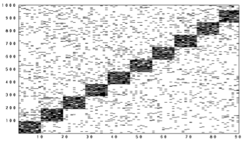
To train the network, we then turned on groups of neurons in order: this was a sequence of 10 neurons at a time, turned on for 10 time ticks each. This is like telling the network the sequence "A,B,C,D,E,F,G,H,I,J".
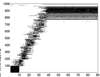
Here's a picture showing what happens in the network at first when training the network as we activated blocks of neurons. In these figures, time moves from left to right. Each little black line means that a neuron was active at that time; to save space, only the part of the network where we "stimulated" is shown. The neurons that we weren't forcing to be active went on and off randomly because of the random connections.
After we exposed the network to the sequence several times, something interesting began to happen. The firing at other times was no longer completely random. In fact, it looked like the network was learning to anticipate that we were going to turn on the blocks of neurons:
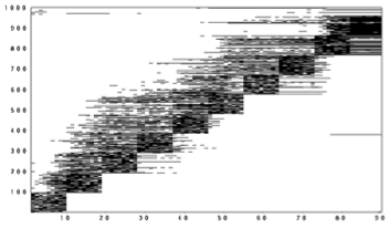
Did the network learn the sequence? Suppose we jumpstart it with "A". Will it remember "B", "C",… "J"?
Indeed it did! A randomly-connected neural network equipped with this synaptic modification rule is able to learn sequences!
This was an example of a "learning rule" and just one function — the ability to learn sequences of patterns — that emerges in a network governed by this rule. In future posts, I'll talk about more about these kinds of models and mechanisms, and their emphasize their relevance to cognitive neuroscience.
-PL
Edit (9:33pm Eastern): Included the current numerical value of the connection weight in all parts of the equations as per a reader's suggestion.
Awesome article. Thanks.
Thank you. Very interesting. Just one point on your explanation of the formula – in your example if W(now) = 0.5 then you should use consistently throughout your formula, otherwise a newbie like me will get confused. W=0.5 + LearningRate x [PRE(past)-0.5]… Unless I am wrong?
No you’ve got it right — to make sure to not confuse the newbies, and to make it as clear as possible, I’ll make that change now! Thanks!
Wow, this post is awesome. I have a similar (but much less clear) set of notes that I review every time I open up the simulation software I use! This is much better.
This is my first time at this blog – very cool stuff! I’ll be adding you to my blogroll.
Excellent post, and excellent paper! I actually read your paper when it came out. As best as I can tell, very few people are thinking about temporal sequencing in neural nets.